Add Lat/Lon Coordinates to GOES-16/GOES-17 L2 Data and Plot with Cartopy
NOAA’s GOES-16/17 satellite data have been made accessible on Amazon AWS’s S3 object storage. These data are stored on the commonly-used NetCDF4 data format and are easy to access in Python thanks to great tools such as xarray and s3fs.
If you’ve worked with GOES data before though, you’ll know that the data coordinates are on a x/y scan grid, not latitudes and longitudes.
But there’s a (relatively) easy way to convert between the GOES x/y coordinates and latitude/longitude as long as you know a few key parameters about the GOES projection. The full mathematical derivation of the coordinate transform can be found here:
While the guide above goes (pun slightly intended) into great detail on the projections and coordinates of the GOES satellite, I wanted to combine that information with information on how to access the GOES data on AWS, plotting with xarray and cartopy, and put it all in one place.
Code Access
A follow-along Jupyter notebook can be found here:
A Binder environment is also available to run this code interactively on the cloud without needing to set up anything on your local machine. Either click on the badge in the repo’s README file or this link.
To see the code with all the outputs, see here: https://nbviewer.jupyter.org/github/lsterzinger/goes-l2-latlon-tutorial/blob/main/tutorial-with-outputs.ipynb
Let’s go!
First, import the necessary libraries. We’ll be opening GOES data on Amazon Web Services’ S3 storage, so we need s3fs as well as xarray to open the data. We also need numpy for some extra array operations and matplotlib.pyplot for plotting.
We’ll also import cartopy.crs and cartopy.feature for mapping and border options on our plot
import xarray as xr
import s3fs
import matplotlib.pyplot as plt
import numpy as np

import cartopy.crs as ccrs
import cartopy.feature as cfeature
Let’s open the file. We’ll use s3fs and xarray to open the remote file on S3 and convert it into a dataset that we can use for plotting.
fs = s3fs.S3FileSystem(anon=True)f = fs.open("s3://noaa-goes17/ABI-L2-MCMIPC/2021/050/18/OR_ABI-L2-MCMIPC-M6_G17_s20210501801176_e20210501803549_c20210501804089.nc")ds = xr.open_dataset(f)
The ds dataframe has coordinate dimensions x and yin radians, which are part of the GOES projection. Converting these to latitude and longitude is useful for selecting subsets of the data over certain geographical areas.
Do the conversion
This can be accomplished using a bit of math, which I got from this blog post. The math is dependent on some projection parameters, which are stored in the variable goes_imager_projection . The function below uses those parameters, along with the transform math, to return a dataset with lat and lon as xarray coordinates.
def calc_latlon(ds):
    # The math for this function was taken from
    # https://makersportal.com/blog/2018/11/25/goes-r-satellite-latitude-and-longitude-grid-projection-algorithm    x = ds.x
    y = ds.y
    goes_imager_projection = ds.goes_imager_projection

    x,y = np.meshgrid(x,y)

    r_eq = goes_imager_projection.attrs["semi_major_axis"]
    r_pol = goes_imager_projection.attrs["semi_minor_axis"]
    l_0 = goes_imager_projection.attrs["longitude_of_projection_origin"] * (np.pi/180)
    h_sat = goes_imager_projection.attrs["perspective_point_height"]
    H = r_eq + h_sat

    a = np.sin(x)**2 + (np.cos(x)**2 * (np.cos(y)**2 + (r_eq**2 / r_pol**2) * np.sin(y)**2))
    b = -2 * H * np.cos(x) * np.cos(y)
    c = H**2 - r_eq**2

    r_s = (-b - np.sqrt(b**2 - 4*a*c))/(2*a)

    s_x = r_s * np.cos(x) * np.cos(y)
    s_y = -r_s * np.sin(x)
    s_z = r_s * np.cos(x) * np.sin(y)

    lat = np.arctan((r_eq**2 / r_pol**2) * (s_z / np.sqrt((H-s_x)**2 +s_y**2))) * (180/np.pi)
    lon = (l_0 - np.arctan(s_y / (H-s_x))) * (180/np.pi)

    ds = ds.assign_coords({
        "lat":(["y","x"],lat),
        "lon":(["y","x"],lon)
    })
    ds.lat.attrs["units"] = "degrees_north"
    ds.lon.attrs["units"] = "degrees_east"return ds
Now, ds has 2D coordinates lat and lon . Unfortunately, xarray doesn’t support using ds.sel() on non-dimension coordinates, and 2D arrays cannot be added as dimension coordinates.
Instead, we’ll write a small function to return the x/y maxima and minima for a given latitude/longitude box:
def get_xy_from_latlon(ds, lats, lons):
    lat1, lat2 = lats
    lon1, lon2 = lons

    lat = ds.lat.data
    lon = ds.lon.data

    x = ds.x.data
    y = ds.y.data

    x,y = np.meshgrid(x,y)

    x = x[(lat >= lat1) & (lat <= lat2) & (lon >= lon1) & (lon <= lon2)]
    y = y[(lat >= lat1) & (lat <= lat2) & (lon >= lon1) & (lon <= lon2)]

    return ((min(x), max(x)), (min(y), max(y)))
Now when we pass ds to this function, we get a new dataset with lat and lon as coordinates.
ds = calc_latlon(ds)Now, if we print ds.coords we see the following coordinates appended to the list:
lat (y, x) float64 53.5 53.49 53.49 ... 14.8 14.8 14.81lon (y, x) float64 -184.4 -184.3 -184.2 ... -112.5 -112.4
These coordinates are 2D arrays of latitude and longitude, with dimensions (y,x)
Take a lat/lon subset
Adding lat/lon as a coordinate allows for easy taking of a subset of the data. First, define a bounding box in latitude and longitude:
lats = (30, 55)
lons = (-152, -112)
Next, use the get_xy_from_latlon() function we defined above to get the x/y max/min for the given latitude and longitude pairs.
((x1,x2), (y1, y2)) = get_xy_from_latlon(ds, lats, lons)Now that we have x1, x2, y1, y2 defined, we can use ds.sel() to take a subset of the data
subset = ds.sel(x=slice(x1, x2), y=slice(y2, y1))Note: the y-slice must be done in order y2, y1 because the y-coordinate is decreasing from left to right so the larger value must be given first.
Plot with Cartopy
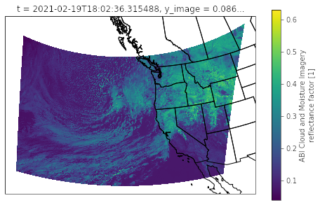
We can use cartopy along with xarray’s built-in plotting tools (built on matplotlib) to plot the imagery on a map. I chose the blue channel (“CMI_C01”) to plot.
p = subset.CMI_C01.plot(
    x='lon', y='lat',
    subplot_kws={'projection' : ccrs.Orthographic(-130, 40)},
    transform = ccrs.PlateCarree()
)p.axes.add_feature(cfeature.COASTLINE)
p.axes.add_feature(cfeature.STATES)
In this example, we define the projection (Orthographic) meaning that the data will be plotted on a globe. The transform (PlateCarree) tells cartopy that the data is in lat/lon coordinates. This yields the following plot:
We can also build a “fake” true-color image by combining the red, blue, and “veggie” channels (GOES does not capture a green band; the vegetation channel can be used instead, but must be corrected else our image would appear too green. For more information, see here)
# Get channels
r = subset['CMI_C02'].data; r = np.clip(r, 0, 1)
g = subset['CMI_C03'].data; g = np.clip(g, 0, 1)
b = subset['CMI_C01'].data; b = np.clip(b, 0, 1)# Apply a gamma of 2.5
gamma = 2.5; r = np.power(r, 1/gamma); g = np.power(g, 1/gamma); b = np.power(b, 1/gamma)# Calculate "true green" from the veggie channel
g_true = 0.45 * r + 0.1 * g + 0.45 * b
g_true = np.clip(g_true, 0, 1)
rgb = np.dstack((r, g_true, b))
Now, we can plot the RGB image with:
fig = plt.figure(figsize=(8,5))
plt.imshow(rgb)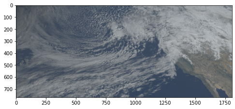
While constructing an RGB image in matplotlib does not allow for plotting on different coordinate grids (so we won’t be able to get coastlines/state borders), we still plotted the following image based on the lat/lon box defined above. For more advanced satellite plotting, see PyTroll/SatPy.
I hope this guide was useful! If you have questions, comments, or suggestions, please feel free reach out to me on twitter @lucassterzinger or via email (see git profile). If you’d like to add something to the tutorial, please feel free to open a PR on the notebook repository.